Group problem for undergrads, individual for grads:
(1) Assume that you are observing stars in a square degree at the NGP, that the thick disk has a scale height of 1 kpc and the thin disk 300 pc, and the halo has an r^-3 density distribution. Furthermore, assume that the ratio of thin to thick to halo stars at the Sun is 1000:100:1 and that the local density of your tracers (halo giants) is 35 per kpc^3. Draw plots of the number of stars per square degree as a function of z height out to 15 kpc. At what distance will the counts of thick disk stars peak? halo stars? (You will need to account for the variation in volume element along the line of sight as well as the variation in star density.)
Individual problem:
(2) The stellar luminosity function
Download the Preliminary version
of the "Catalog of Nearby Stars 3" (CNS3) of Gliese and Jahreiss,
which you can access from
http://vizier.u-strasbg.fr/viz-bin/VizieR?-source=V/70A. This
catalog gives information on all known stars (in 1991) within 25 pc of
the Sun. Within its limitations, this was one of the best
volume-limited samples available in astronomy at that time. Use this catalog to calculate the local stellar luminosity
function in MV. Make sure you download both the parallax
and its error. Things to think about:
(a) There are roughly 3000 stars in
the catalog, but they are not uniformly spread in MV. What might be a good binsize to use here?
(b) For what absolute magnitude ranges is this catalog likely to be
incomplete? Why?
(c) How might you derive the errors on the luminosity function for
each bin?
(d) What units do we usually use for a stellar luminosity
function?
Group problem for undergrads, individual for grads:
(3) In this problem you will use data from the Two Micron All-Sky
Survey to model the distribution of stars in the Milky Way disk.
(a) If you look at the Hipparcos color-magnitude diagram, you can see that
red clump stars are a common type of evolved star. There have been a
number of recent papers which have assumed that all stars in a given
J-K color range are clump stars with the same absolute magnitude
(MK=-1.65) and used the magnitudes of these stars to
estimate their distance distribution along the line of sight.
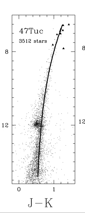
Below is a color-magnitude diagram in the near infrared (K and J-K)
for the globular cluster 47 Tucanae (left, [Fe/H]=-0.7, age ~12 Gyr)

Work out what color range you should use to identify clump stars in the disk using this CMD. You will need to work out the reddening in J-K towards 47 Tuc. Use the compilation of globular cluster properties at http://physwww.physics.mcmaster.ca/%7Eharris/mwgc.dat Transform from E(B-V) to E(J-K) using the transformations in Schlegel et al 1998 (ApJ 500, 525), Appendix B, Table 6.
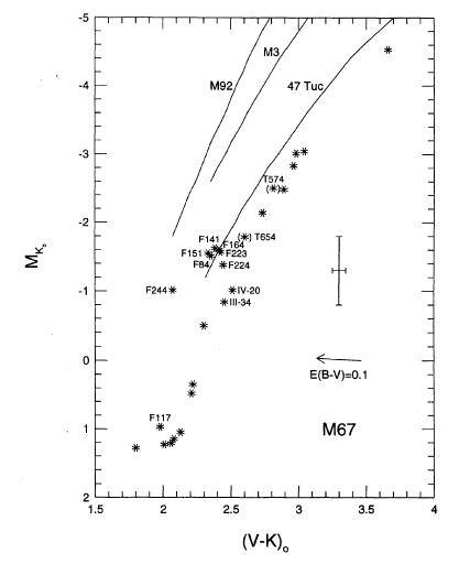
47 Tuc is more typical of the thick disk than the old disk, so also look at the open cluster M67, which has age 2-3 Gyr and roughly solar abundance. Below is a CMD in (V-K)_0 vs M_K for M67.

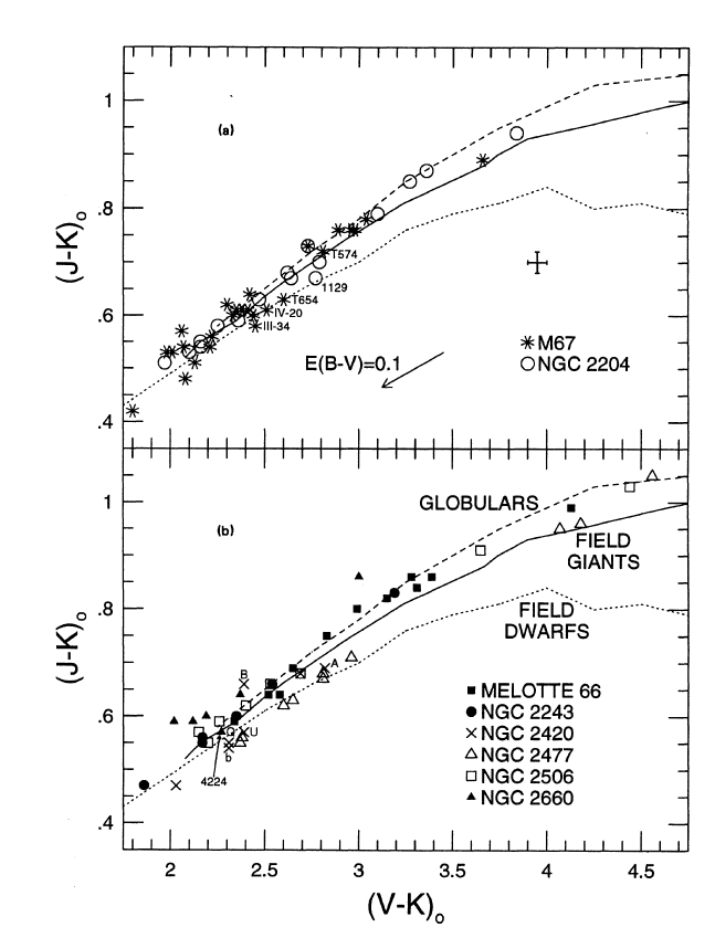
To transform from (V-K)_0 to (J-K)_0, use the top half of the following plot:

What is the color range for the clump in these two clusters in (J-K)_0?
(b) Download some data from the North Galactic Pole to get a feeling
for a field with almost no reddening looks like. You will need to use
the GATOR server, at
http://irsa.ipac.caltech.edu/applications/Gator/.
(Use the 2MASS all-sky point-source catalog. There is a
tutorial for GATOR.) Use the maximum
radius (3600 arcsec), enter galactic coordinates, and download J
and K colors for everything brighter than K=14. Plot K vs J-K. You may
need to download more than one such field to get enough stars in this
low-density region.
Explain the broad features you see in this diagram, and what
evolutionary states are likely to dominate in each region.
(c) With MK=-1.65, and K magnitudes from say 8 to 14, what distances are probed in the Galaxy?
(d) Choose a low-latitude line of sight with a low reddening. Use the maps of Burstein and Heiles (AJ, 87, 1165, 1982) to find a good field. Download data from this direction, calculate distances for each clump star in the sample, and plot a histogram of distances for the stars.
(e) (Graduate students only) Using a double exponential disk model for the Milky Way thin disk with realistic estimates for scale length and scale height, predict how the number of stars should vary with distance along the line of sight. Give the equations you use to connect l and b and distance to galactic X,Y,Z coordinates. How good a fit is the model to the data? You should only worry about the variation along the line of sight, not the absolute normalization of number of stars.
(f) (Grad students only) Are there any assumptions that we have made above that are likely to produce significant errors? Explain why. For extra credit: can you suggest another region of the CMD which might work better than the clump?